Demand & Supply

uni/economics COR2100 Economics and Society

Demand and Supply

Important

The main workhorse model of economics.

• workhorse: main reference
• model: a simplified description of reality

Learning objectives

1. Illustrate how buyers & sellers behave using demand & supply curves
2. Understand how the market works as an allocation mechanism (who gets what)
3. Use demand and supply analysis to predict changes in the market
4. Evaluate market outcomes

Background

Markets

• markets: an arrangement enabling buyers and sellers to trade.
• market price: price at which buyer and sellers conduct transactions
  • in a well-functioning market, contains lots of information
  • given rise to by buyer-seller interaction
• transactions: voluntary; buyers & sellers can turn down any deal

Info

In D&S supply analysis, we assume competition exists on both sides. Both buyers and sellers have options.

Demand & Supply graph

Demand & supply graph

uni/economics

Demand & supply graph

Info

Demand and Supply curves are used to illustrate the behavior of buyers & sellers in market interactions.

Demand curve formula

Demand curve formula

$\text{P}=\text{a}-{\text{bQ}}_{\text{d}}$

• $\text{P}$: price; exogenous variable
  • exogenous variable: a factor whose value is determined outside the economic model being studied
    • influences the system or internal variables but is not affected by them in return
• $\text{a}$: $y$-intercept (choke price)
• $-\text{b}$: slope
• ${\text{Q}}_{\text{d}}$: quantity demanded; endogenous variable
  • endogenous variable: a factor whose value is determined or influenced by other variables inside an economic model

Important

The equation should ALWAYS start with $\text{P}$; use algebra to rearrange if it doesn’t.

Example

$P=7.5-\frac{1}{2}{\text{Q}}_{\text{d}}$

• If P = \8$,$\text{Q}_\text{d}$ is still zero because it’s above the choke price

${\text{Q}}_{\text{d}}=15-2P$ if and only if $0\le P\le 7.5$.

Link to original

• P to D: buyers
• 0 to S: sellers
• P: price
  • the quantity buyers want to buy = quantity sellers are willing to sell
  • at other points, these aren’t aligned → pressure on price to increase or decrease
• intersection: equilibrium of the market
• asterisks: equilibrium
  • “P star” or “P prime”

Info

This is a static snapshot of the market; markets are dynamic.

Link to original

Demand & supply analysis

uni/economics

Demand & Supply analysis

• show how markets change over time
• shed light on puzzling observations about the market
  • e.g. housing going up; computers getting cheaper despite more advanced tech
• but not applicable to all settings
• used for perfectly competitive markets

Link to original

Perfectly competitive markets

Perfectly competitive markets

uni/economics

Perfectly competitive markets

Characteristics

1. Many buyers and sellers, all of whom are so small in relation to the market that no individual buyer or seller has the power to influence the equilibrium price/quantity
   • but a collective action taken by many buyers or sellers will have an impact
2. All sellers sell identical products or services
   • buyers don’t care about who they buy from; they only care about price → sellers cannot raise prices without risking loss of customers
   • the risk is that prices decline when taking products to market (“price takers”)
   • farmers combat this through grain storage – temporary storage of grain to sell when the market improves
     • watch this youtube video
3. There are virtually no barriers to entry or exit
   • they can leave markets that are no longer profitable
   • can easily employ resources elsewhere
   • easy access to labour, capital, other resources necessary to enter market
4. Buyers and sellers are well-informed
   • sellers know if there are better ways of doing things/better opportunities elsewhere
   • buyers know where the prices are lower

---

• every buyer pays and every seller charges the same market price
• information on prices travel costlessly and instantly → buyers know if prices are lower elsewhere
  • buyers will buy from the lowest price
• no seller or buyer is big enough to influence the market price
• all sellers sell an identical good or service

Concept Check

Thinking time

Are petrol stations and/or agricultural markets perfectly competitive?

• my attempt: Neither – big corporations dominate both and decide prices for us
• answer: Agricultural markets are closer
  • coffee, sugar, wheat are traded in exchanges with centralised market prices
    • brokers, sellers, buyers have transparent prices
  • they approximate perfectly competitive markets closely
  • BUT some agricultural products are industrial → some buyers have more bargaining power than others
    • e.g. star anise has high demand becaause of Roche, which makes the Tamiflu vaccine
      • big buyer → lower prices for them → not perfectly competitive
  • wheat as a perfectly competitive market held truer in the days of family farms than massive agricultural industries
  • there’s lots of “apples”, which makes the market not homogenous – unlike copper or gold
  • even accounting for similar locations, brands have different prices
  • buyers believe petrol brands are distinct, maybe because of advertising
• petrol stations are retail stores, and retailers have different prices based on location
  • in a perfectly competitive market, products are identical and buyers buy based on the lowest price (aka best value for them)
• almost no real market satisfies the assumption
  • BUT predictions are still useful
  • it’s a good benchmark for other markets
• Demand & supply analysis can be used for markets close to perfectly competitive

Link to original

Demand

Demand

uni/economics Demand & Supply

Demand

Learning objectives

1. Understand the “Law of Demand”
2. Learn how to draw the demand curve
3. Learn how to “interpret” the demand curve

Case Study: Petrol

• not perfectly competitive
• assume that there are no brands, take petrol as a broad category
  • simplifications like these help get a handle on reality in economics → more confidence in analysing the more complicated version later on

Question

What factors lead consumers buy more or less petrol?

• my answer
  • ✅ price – lower price → more purchase
  • usage of petrol (i.e. are they commuting more? commuting further distances?)
• purchase of cars
• price of petrol substitutes; if cheaper, buyers will trend towards these over petrol
  • e.g. natural gas, diesel, electricity
• Population
• income
• environmental concerns
• expectations of future petrol prices

Summary

If none of the other factors change, there’s an inverse relationship between the quantity of petrol bought and the price of petrol.

Law of Demand

Law of Demand

uni/economics Demand & Supply

Law of Demand

Quote

All else held constant, the lower the price of a good, the higher the quantity demanded; the higher the price, the lower the quantity demanded.

• ceteris paribus: all else held constant (Latin)
• quantity demanded: amount of a good buyers are willing to purchase at a given price

Link to original

Demand curve

Summary

The demand curve plots the quantity demanded at different prices. (MAY NOT BE LINEAR because it depends on buyer behaviour)

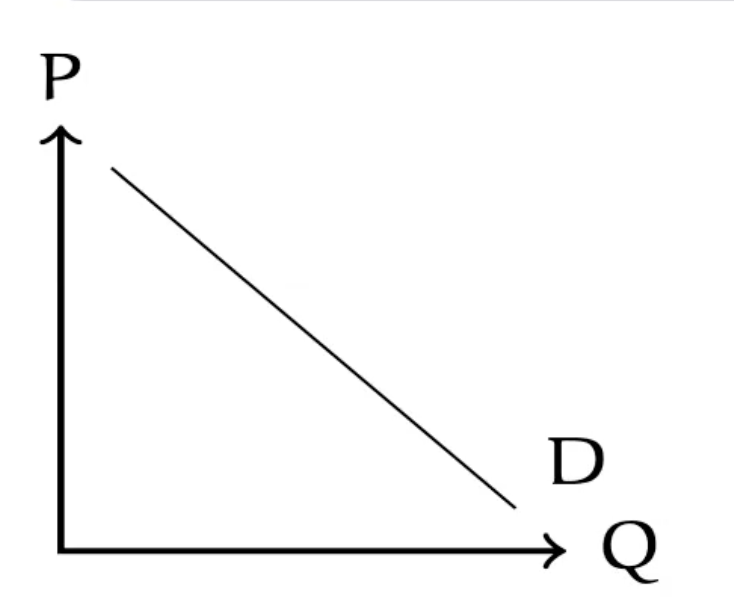
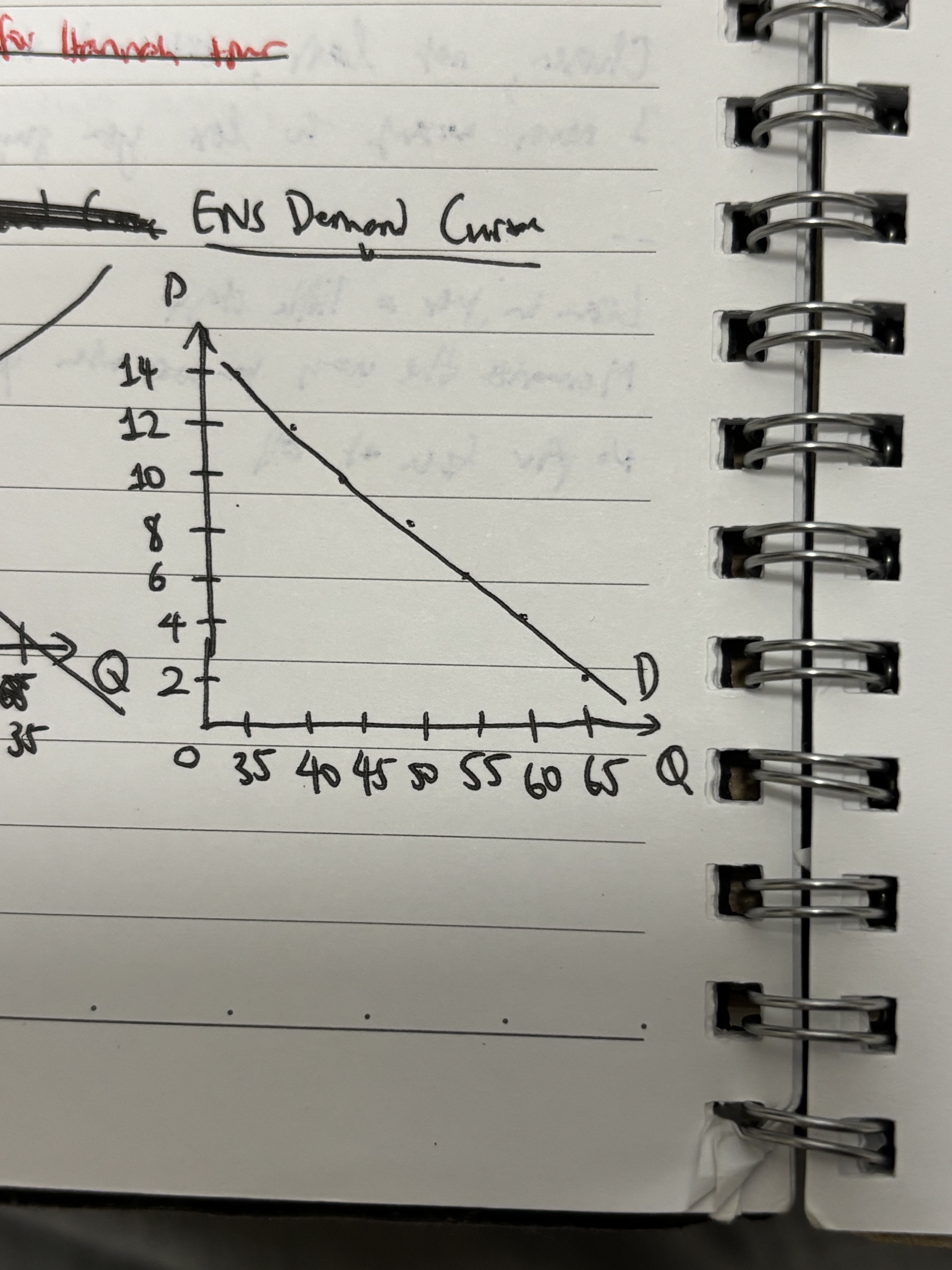
• demand curve is a downward sloping curve (assuming price as y and quantity as x)
  • can be read horizontally; e.g. P = $3.50, $Q_d$ = 10
• willingness to pay: the most someone in the market is willing to pay for a particular unit
  • when you read a demand curve vertically
• when quantity demanded changes along a demand curve, it’s only due to changes in the price
• choke price: the price there is no quantity demanded
• freebie quantity: quantity demanded when price is zero
• demand schedule: table reporting the quantity demanded at different prices, ceteris paribus
  • 
  • it’s a cumulative table; anyone willing to pay $5 is also willing to pay $2
• unit demand: when consumers are only interested in buying ONE unit of the good
  • quantity demanded = number of buyers

Problem 1: Laundry detergent

My answer:

• MISTAKE: x-axis not proportional

Solution:

Why isn’t the price the same for everyone?

$\text{demand}=\text{want an item}+\text{willing and able to pay}$

• a buyer compares WTP with market price
  • if WTP > market price → buy

Horizontal Summation

Learning Objectives

1. Aggregate demand curves using demand schedules
2. Aggregate demand curves using simple math

How-to

Summary

Aggregating individual demand curves to get the total demand curve?

1. Obtain demand schedule
2. Add the demand quantity of each buyer together per row to get the market demand
3. Plot new curve

Using algebra

Demand curve formula

Demand curve formula

$\text{P}=\text{a}-{\text{bQ}}_{\text{d}}$

• $\text{P}$: price; exogenous variable
  • exogenous variable: a factor whose value is determined outside the economic model being studied
    • influences the system or internal variables but is not affected by them in return
• $\text{a}$: $y$-intercept (choke price)
• $-\text{b}$: slope
• ${\text{Q}}_{\text{d}}$: quantity demanded; endogenous variable
  • endogenous variable: a factor whose value is determined or influenced by other variables inside an economic model

Important

The equation should ALWAYS start with $\text{P}$; use algebra to rearrange if it doesn’t.

Example

$P=7.5-\frac{1}{2}{\text{Q}}_{\text{d}}$

• If P = \8$,$\text{Q}_\text{d}$ is still zero because it’s above the choke price

${\text{Q}}_{\text{d}}=15-2P$ if and only if $0\le P\le 7.5$.

Link to original

Find the gradient: $\frac{\text{rise}}{\text{run}}$

TODO Problem: Find Carlos’s demand curve

Demand curve shifters

Demand curve shifters

Learning Objectives

1. Understand what a shift in the demand curve means
2. Enumerate common factors that shift the demand curve in each direction

Summary

Demand curve shifters are factors that shift the demand curve either left or right.

Important

• Movement along the curve → price changes
• Shift along the curve → change in non-price factors

Left right left right swing it to the beat –Strategy by Twice

• LEFT
  • factor causes quantity demanded at each price to decrease; ${\text{Q}}_{\text{d}}$ falls → whole demand curve shifts to the left
  • decreases willingness to pay
  • e.g. KitKats – presence of substitutes, preference for healthier snacks, less pocket money
• RIGHT
  • factor causes quantity demanded at each price to increase → whole demand curve shifts to the right → higher willingness to pay
  • this is by quantity of good consumers want to buy, regardless of price
  • e.g. KitKats – students hungrier after a 5-hour class, more money for discretionary food items, no substitutes available
• monotonic: if you like a good more, it shifts; if you like it even more, it shifts in the same direction

Common demand shifters factors

• availability of substitutes
• preference
• changes in prices of substitutes (‘in place of’)
  • cheaper substitutes → consumers buy those → less demand for the OG Product A
  • more expensive substitutes → consumers go to Product A
• price/availability of complements (‘together with’)
  • e.g. laptops & software going hand-in-hand
• number of buyers (population)
• income of buyers
  • income ↑ = demand for NORMAL GOOD ↑ (most goods – e.g. household appliances, food, clothes)
  • income ↑ = demand for INFERIOR GOOD ↓ (instant noodles, canned meals)
  • neutral goods: regardless of income, e.g. you wouldn’t buy lots more toothpaste if you became a millionaire tomorrow
• expectations about the future
  • ↓ expectations = ↑ demand
    • e.g. price to increase, or scarcity
  • ↑ expectations = ↓ demand
    • complacency that product is always going to be there

Testing hypotheticals

1. Determine which curve it shifts
2. Determine what factors, if any
3. Determine which direction it moves

Link to original

Link to original

Lecture notes

Curve shifting in Equilibrium

• comparative statics

Supply

Supply curve shifters

Supply curve shifters

uni/economics Supply

Supply curve shifters

Refer to the Law of Supply

Common factors

• number of sellers
• input prices: cost of production
• technology: how it’s produced
• seller’s expectations about the future
  • expectations: any belief inducing action
  • ↓ expectations = sell now rather than later
  • ↑ expectations = sell later rather than now

Link to original

Willingness to accept

• willingness to accept: the least amount of money accepted in return for supplying one more unit to the market ($y$-axis)

Marginal cost

marginal cost

marginal cost

Summary

The extra cost a business pays to make one more unit of a product.

• if 10 toys cost $100 to make and 11 cost $108, the marginal cost is $8

Formula

$$\text{marginal cost}=\frac{\text{change in total cost}}{\text{change in quantity}}$$

Applications

• mostly variable costs like raw material and labour
• fixed costs like rent don’t change by quantity of product made

Relevance

• finding profit limits – companies maximise profit when marginal cost = marginal profit
  • marginal profit: extra money made from selling that one item
• spotting efficiency
  • early on, making more items can lower costs due to efficiency
  • later, costs rise because of crowding or tired workers – diminishing returns

Link to original

REVIEW

Analysing changes in equilibrium

1. Decide if the event shifts supply or demand or both
2. Determine the direction the curve shifts
3. Use supply-and-demand to see how the shift changes equilibrium price and quantity